ML lesson 2

[back] [code download]

To set up your code on Mac or Linux, open the terminal and run:

curl -LsSf https://h.sherstnev.org/setup2.sh | sh

On Windows, open powershell and run

powershell -ExecutionPolicy ByPass -c "irm https://h.sherstnev.org/setup2.ps1 | iex"

Summary

We trained a classifier that takes as input sensor data from a smartphone and predicts the activity that the person is doing. We used a very similar neural net to last time, with some new techniques.

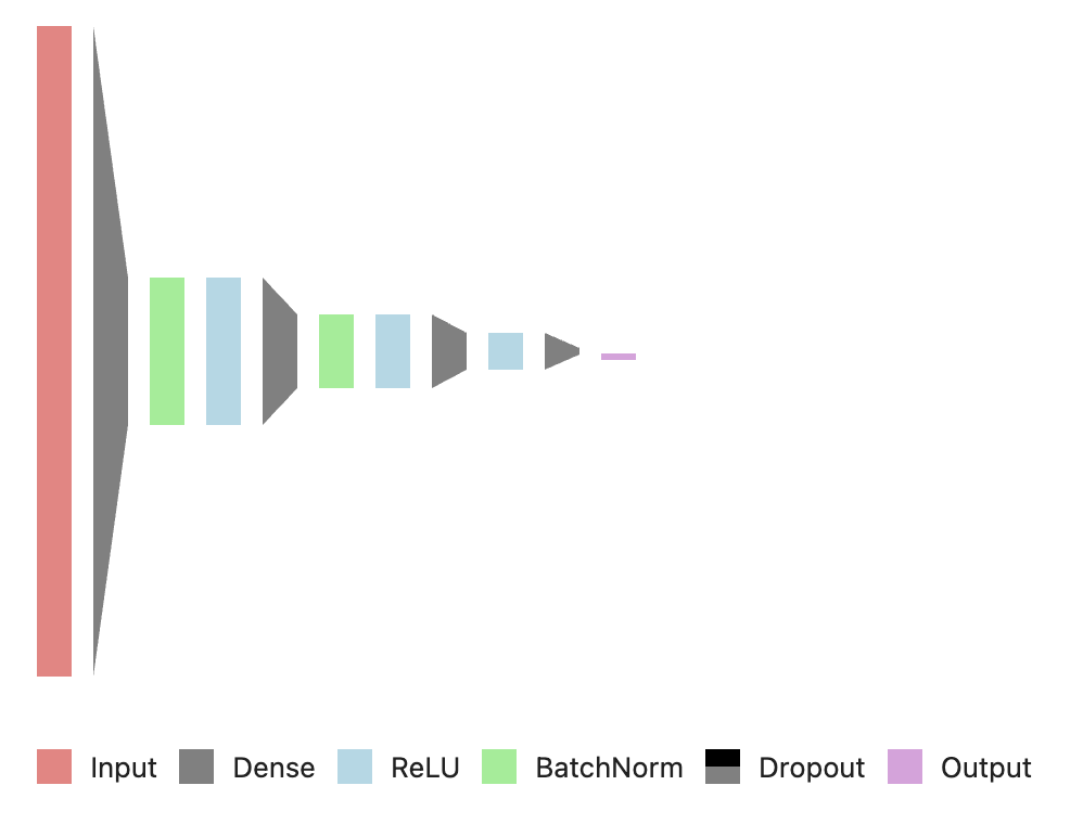
We ended up with the network:

model = nn.Sequential(
    nn.Linear(num_features, 128),
    nn.BatchNorm1d(128),
    nn.ReLU(),
    nn.Dropout(0.3),
    
    nn.Linear(128, 64),
    nn.ReLU(),
    nn.Linear(64, 32),
    nn.ReLU(),
    nn.Linear(32, num_classes)
)

Review from last lesson:

1. What is a neural network
2. Loss
3. Optimizer searches for parameters that minimize loss through backpropagation
4. Activation functions (ReLU)

New topics:

1. Categorical activation & loss
   1. Categorical crossentropy
2. Batching
3. Batch normalization
4. Dropout
5. How batch size, normalization, dropout, and learning rate affect training rate, stability, and overfitting

How parameters affect training

1. Learning rate
   1. higher learning rate -> less likely to get stuck in local minima, might converge faster
   2. lower learning rate -> more stable training, might not overshoot the best parameters
2. Batch size
   1. higher batch size -> smoother training, can be faster, sometimes can overfit more
   2. smaller batch size -> less stable training, can be slower, sometimes prevents overfitting
   3. best batch size depends on the number of features you have. Often you should choose a power of 2
3. Dropout
   1. larger dropout -> can prevent overfitting, but slows convergence. Often you should just reduce the number of parameters instead of adding dropout
   2. smaller/no dropout -> generally preferrable if the model doesn't overfit, but not possible for some networks
4. Batch normalization (BatchNorm1d)
   1. BatchNorm sometimes makes convergence way faster

Softmax activation / Why we use log likelihood

Models are good at adding things: each neuron is a weighted sum of its inputs. Probabilities mostly compose by multiplying, though: "probability that A happens AND B happens" = $p(A) \times p(B)$.

We want the neural network to model probabilities in a way that adding numbers corresponds to multiplying probabilities.

We treat the numbers that come out of the neural network as log likelihoods, since $\log a + \log b = \log (ab)$. Then, we use the softmax activation function to turn them into a probability.

For each output from the model $x_i$, we compute a probability $$p_i = \frac{\exp x_i}{\sum_j \exp x_j}.$$

We showed that adding up these $\sum_i p_i = 1$, and that each $0 \le p_i \le 1$.

Loss function: categorical crossentropy

The loss function we used is called "categorical crossentropy":

1. "Categorical" because it's useful for when the output says which category the input is in
2. "Entropy" is a measure of disorder, and the loss measures the disorder in the predicted probabilities
3. "Cross" because it's the disorder between the predicted probabilities and the expected category

Weirdly mathy name for something that's not that complicated:

$$ L = - \log (\text{predicted probability of the expected output}). $$

PyTorch reference [here].

"Homework"

Try one of these:

1. Improve test accuracy to >96% while keeping the test-train gap <2%; or
2. Improve test accuracy >97.5%

Both are possible with what we learned. Again best model (best performance + most interesting approach) gets a prize on Wednesday.